Evidence-based physical examination: sensitivity and specificity (part I).
Posted on 30th September 2013 by Donatas Zailskas

In clinical practice you have two main responsibilities: to determine the right diagnosis and to assign the correct treatment. This means the diagnostic tests you are using must be as accurate as possible. This way you can categorize patients as high or low risk for a certain disease and not choose blindly. When I speak of diagnostic tests, I do not only mean laboratory tests or imaging studies – you are the most important diagnostic test there is! However, a lot of physical examination points are not as useful as you’d think, yet still taught as something of high importance in clinical practice.
In order to eventually get to the Evidence-Based Physical examination, we must first begin with the concepts of sensitivity and specificity. This table is the so called Bayesian square and it is a brief visualization of how you can figure both of them out:
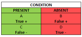
The Bayesian Square
When we talk about sensitivity and specificity, you should set your mind that “Has the condition” and “Does not have the condition” are the default starting points, not “Tests positive” and “Does not test positive”, about which we will talk in the following blog post.
The green column in the Bayesian square represents the total number of patients who you know have the condition, including those who have the condition, but test negative (a false negative). The red column represents the total number of patients who you know do not have the condition, even though amongst them there are patients who test positive (a false positive). It is obvious, that false negatives and positives should be avoided as much as possible – in the first case you can underdiagnose a patient and abstain from so needed treatment, and in the latter case you can get faulty information about the patient’s condition and subject them to a battery of unnecessary diagnostic tests or treatments.
Sensitivity (SN) is the green column – the proportion of patients with the condition who have a positive test. You can count the SN by dividing the number of patients who you know have the condition and test positive, by the total number of patients – those who have the condition and test positive, plus those who get a false negative even though they are ill: A/(A+C). From this equation you can see, that SN rises if the number of false negative test results decreases (C goes down).
Taken from Wikipedia
Let’s say you tested a bunch of people and now have 100 patients who you know have the condition and tested positive for it (A) using a diagnostic test that has 60% SN for that condition. How many patients might not have gotten a treatment for that condition in the process because of all the false negatives? Well, 100/(100+C) = 0.6, so C is roughly 66.7 patients. This means that if you get the right diagnosis for 100 people, 66.7 are underdiagnosed in the process (1 false negative for every 1.47 true positive). Now let’s do the same example when the SN is 90%. In this case, the number of false negatives (C) is only roughly 11.1 patients, and that means that the ratio changes to 1 false negative for every 9 true positives.
Let’s look at it from a different angle. Now you have a total of 100 patients tested – not tested positive for a condition you know they have, but just tested positive in general (A+C). The SN is the same, 60%. How many did you miss this time? Well, the number of patients tested positive for a condition they actually have this time is 60, so C is: 100–60=40. Again, let’s do this with a 90% SN. The number of patients tested positive for a condition they actually have is 90, and the number of false negatives is 10. The ratio of 9 to 1 is more evident.
Right, on to the specificity (SP)! Here’s the Bayesian square again so you wouldn’t have to scroll up.
The Bayesian Square
SP is the red column – the total number of patients without the condition, including those who test positive despite being healthy. In other words, it is the proportion of patients without the disease who have a negative test. SP, unlike SN, protects from overdiagnosing with false positive when there actually is no disease. SP can be counted by dividing the number of patients who you know do not have the disease and actually test negative for it (D) by the total number of patients tested, including those who you know do not have the condition, yet test positive (false positive) . SP rises if your diagnostic test gives as few false positives as possible (B drops).

Taken from Wikipedia
Let’s say you tested a bunch of people with your new fancy diagnostic test and now you know, that now you have a total sample size of 100 patients who tested negative for a condition you know they do not have (D) using a diagnostic test that has 60% SP. How many people got a false positive result as collateral damage in the process? Well, D = 100, so B + D is roughly 166.67 patients and B is about 66.7 patients. So in the process of testing your new diagnostic test you gave about 67 patients a faulty diagnosis. Now if you would have done that with a diagnostic test that has 90% SP, the amount of false positives would be only about 11 people. A different example again would be with a total of 100 patients tested using a diagnostic test with 60% SP (just tested, not tested negative for a condition they do not have). This means B + D = 100, so D = 100 x 0.6 = 60 people. So if you just test a hundred people with you new flashy diagnostic test, 60 of them will get the right result, but 40 will get a false positive result. And if you do the same with 90% SP, only 10 people out of 100 will get a false positive.
All this sounds great when you have the actual percentages, but how do you know if they’re good enough? How do you know that a patient being tested actually has/doesn’t have the condition (actually is A/D), if you’re trying to find out if he has that condition with the diagnostic test of your choice? Well, we go backwards here: the diagnosis was made using something else; SN and SP are designed to assess how well a new diagnostic test compares to what is considered the gold standard – a test that is considered the definitive approach for diagnosing a disease without, ideally, missing a disease or falsely labeling someone as sick.
* * *
So all in all, a high SN is simply a way to protect you from a false negative when there actually is a condition. But here’s a twist – a negative result from a highly sensitive test can rule a diagnosis out: SnNOut (Sensitive, Negative, Out). If you get a negative test result, there’s only a very small chance that it is a false negative, so you can safely accept it as a true negative and dismiss the condition. A high SP, on the other hand, makes sure that, if you do not have the disease, we could actually assure you that you do not have that disease, not give you a false positive test result. And in a similar manner, high SP allows you to rule a diagnosis in: SpPIn (Specificity, Positive, In), because a positive result from a highly specific test means there’s a high chance the positive result is true positive, not a false positive. Even though these mnemonics are useful in remembering what SP and SN are, they are inferentially misleading, as SN and SP are not superior to each other! The diagnostic power of any test is determined by both SP and SN. If you use a diagnostic tool that has a high SN, but a low SP, yes, you will rarely miss a diagnosis for a patient who actually has the condition of your interest, however, you will also overdiagnose a lot of patients due to many false positives from a low SP. In a different situation, if you use a diagnostic tool that has a low SN, but a high SP, you will often miss patients who have the disease, even though you will avoid mistakenly overdiagnosing patients due to a high SP.
The last thing you should keep in mind is the elephant in the room: you must always critically appraise the studies that the sensitivities and specificities were counted in. These studies could be affected by all sorts of problems. First of all, a diagnostic study can be too small to define the test’s performance with sufficient precision. Second, a number of possible biases can be introduced, i.e. spectrum bias. It arises when the patients in the study do not represent the population seen in practice: tests can simply be evaluated in patients known to have the disease and free of it, excluding those with borderline or mild expressions of the disease and conditions mimicking it. This leads to exaggeration of both SN and SP. Another bias, partial verification bias, arises when the gold standard test is not applied consistently to confirm the results of the new test. Incorporation bias might arise when the test under evaluation is also the part of the reference test, obviously overestimating the accuracy. Another problem is that the performance of the test varies considerably from one setting to another. This can happen even for the slightest reasons ranging from simple differences in the definitions of the disease to different interpretations of test results in high and low risk patients.
Conclusion
So, let’s recap:
- Sensitivity is the proportion of people with the disease who are correctly identified by a positive test result, and a negative test result from a highly sensitive test can rule a diagnosis out (SnNOut);
- Sensitivity and specificity are designed to assess how well a new diagnostic test compares to the gold standard;
- Specificity is the proportion of people free from the disease who are correctly identified by a negative test result, and a positive test result from a highly specific test can rule a diagnosis in (SpPIn);
- The power of a test to rule a diagnosis out does not depend exclusively on its sensitivity, and is reduced by low specificity. Similarly, the power to rule a diagnosis in depends on both specificity and sensitivity as well;
- Don’t take sensitivity and specificity for granted – studies quoted as showing SpPIn and SnNOut properties must be critically appraised for possible methodological flaws and biases;
SP and SN might seem similar, so you need at least a little practice to not mix them up. This is the part where you take a deep breath, look through the Bayesian square again, make a few notes, your own examples and get some coffee, because we’re just getting started.
References:
- Pewsner D, Battaglia M, Minder C, Marx A, Bucher HC, Egger M. Ruling a diagnosis in or out with “SpPIn” and “SnNOut”: A note of caution. BMJ. 2004;329:209–213;
- McGee S. Evidence-Based Physical Diagnosis. 3rd ed. Philadelphia, PA: Elsevier Saunders; 2012. Part 2, Understanding the evidence; p. 7-41.


No Comments on Evidence-based physical examination: sensitivity and specificity (part I).
Great article.
9th June 2019 at 12:52 amIs this a typo?: “Let’s look at it from a different angle. Now you have a total of 100 patients tested – not tested positive for a condition you know they have, but just tested positive in general (A+C).”
From the chart, I think this should be (A+B). A is true + and B is false +. On the other hand, (A+C) would be all the people who actually have the disease.