Linear regression: a practical introduction

Posted on 29th August 2017 by Saul Crandon

The following blog article has been written to provide an overview of linear regression. It is suitable for those with little to no experience of this type of analysis. This is not a guide on how to conduct your own analysis, but instead will serve as a taster to some of the key terms and principles of regression. Further reading resources will be provided at the end for those who wish to further their knowledge.

Correlation vs Regression

Like regression, there are different types of correlation. The main two types of correlation are Pearson’s correlation and Spearman’s correlation. Pearson’s correlation focuses on describing a linear relationship between two variables, whereas Spearman’s correlation is more concerned with the rank-order of the points, regardless of where exactly they lie.

Furthermore, it is important to distinguish correlation from regression:

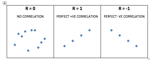
• Correlation is a statistical technique that describes the strength of a relationship between two variables, given as a correlation coefficient, r. It doesn’t matter which variable is x and y, the correlation coefficient is always the same. The value of r has a possible range from -1 to +1 (1). The following plots illustrate the appearance of different correlation coefficients.

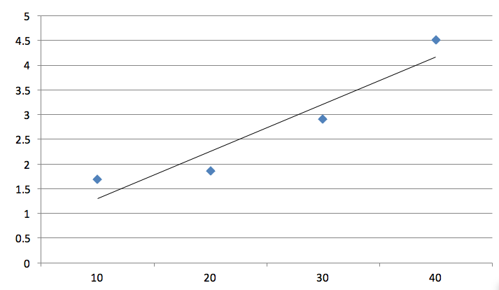
• Regression also describes relationships between variables. However, in regression, a change in one variable is associated with changes in another variable. The result of linear regression is described using R². Regression analysis involves creating a line of best fit. This is described mathematically as y = a + bx. The value of ‘a’ is the y intercept (this is the point at which the line would intersect the y axis), and ‘b’ is the gradient (or steepness) of the line. This is useful as once this line is created, you can predict values of y (or the dependent variable) based on values of x (or the independent variable). This line of best fit is used to summarise the relationship between the variables as shown below.

A few similarities between correlation and regression should also be noted. Most importantly, neither can affirm causality (2). This is because although a change in x might result in a change in y, it is possible that both variables are related to a third confounding variable not described in the analysis. Secondly, the square of Pearson’s correlation coefficient (r) is the same value as the R² in simple linear regression.

Simple vs Multiple Linear Regression

Simple Linear Regression

One variable is dependent and the other variable is independent.

Regression results are given as R² and a p-value. R² represents the strength of association, whereas the p-value is testing the null hypothesis, that there is no association between the variables. Therefore, if the resulting p-value is low (usually defined as < 0.05), we can assume that the relationship between the variables is unlikely the result of chance and so, we reject the null hypothesis.

Multiple Linear Regression

One dependent variable and two or more independent variables.

Multiple linear regression follows the same concept as simple linear regression. However, the difference is that it investigates how a dependent variable changes based on alterations in a combination of multiple independent variables. This reflects a more ‘real-life’ scenario as variables are usually influenced by a number of factors.

The general process of multiple linear regression is as follows (a backwards elimination method is used in this example):

• An outcome (or dependent) variable is defined
• Two or more independent variables are defined
• All variables enter the model and the analysis is run
• Non-significant variables (P > 0.05) are removed and the analysis is re-run
• To validate the final model, residuals are calculated and plotted to assess linearity of the data
• If the assumption of linearity is met then the model is complete
• The model may be adjusted to optimise its suitability

The removal of non-significant variables is important and can be done most commonly with either forwards or backwards elimination methods (2). Forwards elimination means you remove these variables before the analysis is run whereas backwards elimination does this after the results are obtained. The non-significant variables can be removed if their absence from the model would not significantly decrease the effectiveness of the model. Removing these improves the models ‘goodness-of-fit’. Variables with low p-values (P < 0.05) remain because this implies they are meaningful additions to the model and that changes in them are associated with changes in the dependent variable. A model is finalised when no more variables can be removed without a statistically significant loss in fit.

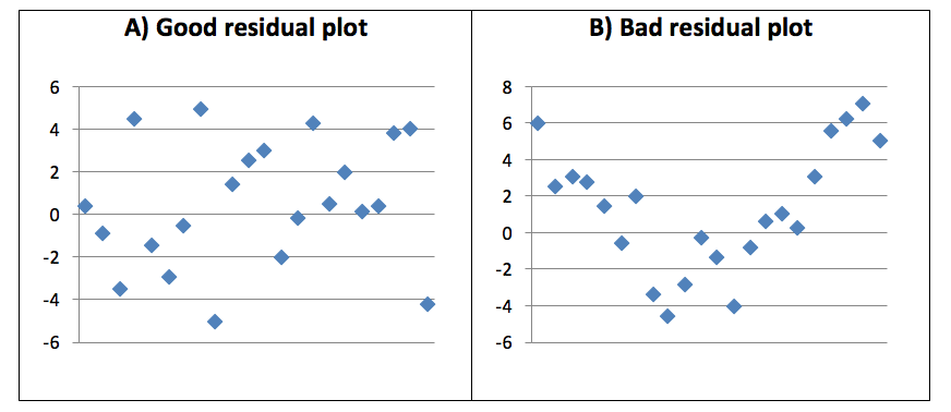
Residuals are the difference between the observed and predicted value of the dependent variable (y). Residuals are crucial, as this allows the model to be validated. Residuals must be calculated for each data point, plotted and then inspected to verify the suitability of the model. The points on a residual plot should have an even distribution around the horizontal axis of zero. If so, the assumption of linearity of the data is true and it is suitable for its intended purpose. A bad residual plot is when there is clear pattern to the data. In other words, the residual data points are skewed. The following graphs show a good and bad example of residual plots.

If the residual plot looks less than ideal, data transformations can be conducted. The methods of doing so are beyond the scope of the article, but in short, it allows the non-linear data to be used more effectively with the linear regression models. It is important to always state if any data transformations were performed.

Once the model is complete, it should be tested on further independent data sets to check its suitability (i.e. data that was not used to construct the model itself). A developed model can be shown to be robust if it is still effective with independent data.

Finally, it is always important to state clearly if there was any missing data. Complex methods do exist to handle missing data sets in linear regression, but these will not be discussed here.

An example of a multiple linear regression model is shown below in the form of both a table and the resultant equation.

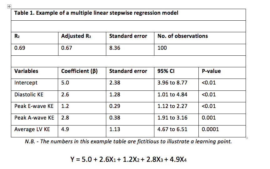
Firstly, the table shows all the necessary components of the model. The R² value is given here; however it is good practice to use the adjusted R² value, as it accounts for the sample size used.

The equation shows the line of best fit. It expands upon the y = a + bx formula to account for the multiple independent variables involved.

A few assumptions needed for Linear Regression

• The number of observations should be greater than the number of x (independent) variables.
• There should be little to no multicollinearity (this will be discussed in the next section).
• The residual plots are evenly distributed around the horizontal axis of zero, i.e. the mean of the residuals is close to zero. This means the data is linear.

A few problems with Regression

Poor fit (over-fitting, under-fitting etc.) of a model means it does not serve it intended purpose effectively. There are ways that the model can be adjusted to optimise its usefulness.

Multicollinearity exists when two or more of the independent variables in the model are highly correlated with one another. This poses a problem as these related variables offer much the same information to the model. To deal with multicollinearity, one of the variables must be removed (usually the least significant one/highest p-value). The Variance Inflation Factor (VIF) is calculated for each independent variable and is used to determine whether multicollinearity is present. Basically, a high VIF means the variable is explained by other independent variables, whereas a low VIF means it is not. A low VIF is good and indicates no significant multicollinearity. It’s important to clarify that no universal cut-off point exists and so it requires a subjective, but educated decision from the researchers conducting the analysis to determine if the value of VIF is acceptable or not. Regression is an artful science and so, requires informed judgement and experience to optimise a model for its intended purpose.

Summary

Linear regression is a useful method to predict changes in a dependent variable based on alterations in independent variables. It is hoped that this blog can act as a gentle introduction to this type of analysis. For more information about linear regression, the following web resources are recommended:

• Student 4 Best Evidence (S4BE) website – This site has a number of relevant student-written articles.
• YouTube – There is a vast library of useful videos on YouTube from basic introductions, to detailed step-by-step guides to conducting your own regression across a range of programs.
• BMJ website – The BMJ is a reliable source of high quality articles regarding statistics.
• Penn State Eberly College of Science: STAT101 course – This website provides detailed guides on all types of statistics. The following links provide thorough tutorials on simple linear regression: https://onlinecourses.science.psu.edu/stat501/node/250 and multiple linear regression: https://onlinecourses.science.psu.edu/stat501/node/283

References

1. BMJ.com. (2017). 11. Correlation and regression | The BMJ. [online] Available at: http://www.bmj.com/about-bmj/resources-readers/publications/statistics-square-one/11-correlation-and-regression [Accessed 22 Aug. 2017].
2. Schneider A, Hommel G, Blettner M. Linear Regression Analysis. Deutsches Artzeblatt International. 2010 Nov; 107(44): 776–782.

Tags: