Using Measures of Variability to Inspect Homogeneity of a Sample: Part 1
Posted on 24th February 2022 by Tarik Suljic

My previous blog explored how measures of central tendency (MCT) are used in the majority of clinical research papers, and that reporting MCTs means very little, if anything, in the absence of other secondary data. In this two-part blog, I will discuss the basics of measures of variability and explain how we can use these to evaluate data homogeneity further.
The first part will cover named variability measures (variability measures bearing units with them) and the second part will cover unnamed variability measures (coefficient of variation and z-score).
In this blog, you will learn about:
- What homogeneity of a sample is and how to inspect it;
- What internal and external validities are and how to assess them;
- What causes variability and how to measure it;
- Basic concepts of range, standard deviation, and variance and how they help us inspect sample homogeneity, as well as internal and external validities.
What are measures of variability?
Measures of variability are statistical tools that assess data homogeneity thus providing us with information on the quality of the sample middle.
Generally, causes of data variations can be classified into three groups:
- Biological causes are characteristics that are inherent to people and that we cannot change, but may be able to control for in the analysis afterwards. Examples of biological causes are sex, age, and genetics.
- Temporal causes. Results may vary based on when they are acquired. For example, blood glucose results will vary across a day, based on a patient’s daily activities and the physiology of blood glucose control.
- Errors in measurements occur when measuring the same thing with different equipment. For example, two spectrophotometers – machines that can measure a concentration of a substance – that are not calibrated equally will produce inevitable differing blood glucose readings.
Mistakes that encompass these errors, if not taken into consideration, are likely to result in distorted validity and systematic errors, therefore resulting in bias. The validity can be defined as the degree to which measurement and/or study represent true inferences. For a study sample, internal validity may be true; however, the external validity that applies to a certain population, may not be.
For example, if a study of the effectiveness of drug A vs drug B for chronic myeloid leukaemia (which occurs mostly in older people) recruits a high proportion of younger patients, the results that arise from this study may be true for the study sample (internal validity), but the results may not apply to the greater population (poor external validity).
One tool we can use to assess the homogeneity of a study sample are measures of variability. We can split them into two categories: (1) those that have units– measures of variability in a narrow sense and (2) those that do not – coefficients. The examples below are all from the first category.
Range
The easiest of all variability measures is range. It represents a span between the two extreme numbers of a set.
For instance, if a set has entries of 15, 17, 19, 20 and 21, the range would be from the minimum number, 15, and the maximum number, 21. Hence the range is calculated as 21-15=6. Values in a range include the units; for example, kilograms (kg) if we are describing the weight of young children.
A range of 6kg in a study of young children is quite large. If it was an intervention research study, this may introduce bias as these children are likely to demonstrate different physiology. If, however, the research study was about a diagnostic radiographic test, then it would be encouraged to have diverse baseline differences because we need to know that a certain device can detect a certain disease in individuals of different ages.
The important thing is that the range of any dataset is taken into context of the study which the data comes from.
Standard deviation – the most used measure of variability in research
In the simplest terms, standard deviation tells you how spread out the data is. Standard deviation (SD) is a linear measure of how far each observed value is from the mean, and describe it not only as a raw value but as being ‘n-standard-deviations away from the mean.’
How do we calculate standard deviation?
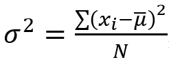
Let’s first imagine that we have a set A={5, 9, 2, 7, 1}. The formula for SD is:
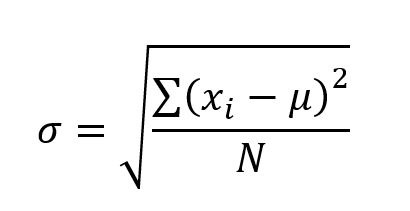
Where σ is SD, xi is a set constituent, μ is the mean, and N is the number of set constituents.
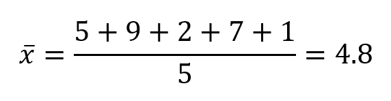
First, we need to calculate the mean by adding up all constituents of the set and then dividing by the total number of set constituents:
Next, we calculate the square difference of each set constituent and then add them all up before dividing with the total number of set constituents, and finally square-rooting it.
The square difference is calculated by subtracting each set constituent from the mean.
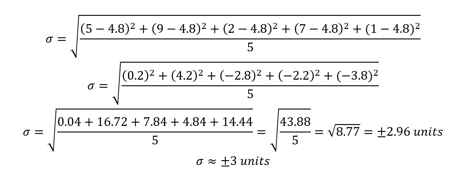
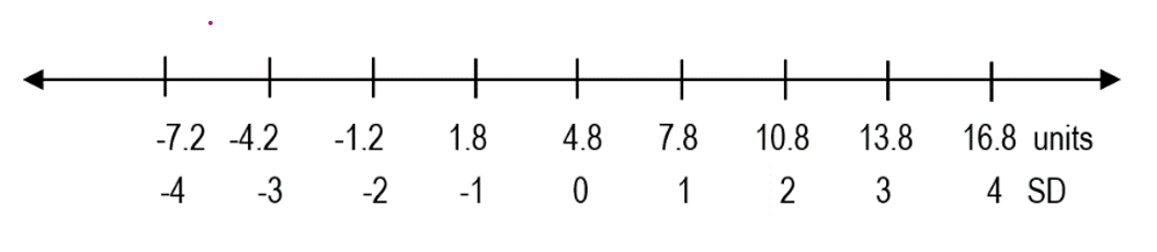
Considering that we obtained (one) SD of approximately ±3 units, we can now draw a numbered line including all the data, and break it down in equal portions, according to the standard deviation.
How do we interpret standard deviation?
We said that SD is a linear measure of spread from the mean. Accordingly, the mean of our dataset is 4.8 units, and the SD is ±3 units. So, anything 3 units above the mean, which is 7.8 units, is 1SD away from the mean. Likewise, anything 3 units below the mean is said to be minus 1SD away from the mean. Similarly, if something is 6 units away from the mean, in either direction, it is said to be ±2-standard-deviations away from the mean.
The greater the standard deviation, the greater the variability of the data.
Why is standard deviation relevant?
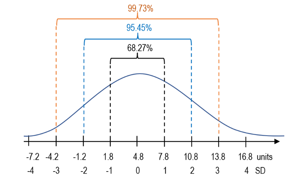
In a total population of students who are being graded 1-5 in several subjects, we expect the majority of them to stick around the (hypothetical) mean, which is 3. Students whose grade point average (GPA) turns out to be either 1 or 5 can be considered as exceptional results. This is true for a normal distribution in which ~68% of sample data is found within 1SD from the mean, ~95.5% within 2SD. Anything above or below 2SD may be considered extreme. Therefore, standard deviation, as a measure of variability, helps us understand where each of our constituents falls under the curve of normal distribution, also known as Gaussian or bell curve.
Variance – the most avoided of variability measures in research
Variance, like SD, describes how distant set constituents are from the mean. However, the key difference is that variance is an average of squared differences from the sample mean, thus informing us about the average degree to which each dataset constituent differs from the mean.
The formula for variance is as follows:
 σ2 is variance, xi is a set constituent, μ is the sample mean, and N is the total number of set constituents. You may think this formula is very similar to the SD formula. That is because variance is SD squared, hence being denoted as σ2.
In the previous section, the SD was ±2.96 units. Should we want to obtain the variance, we just square it.
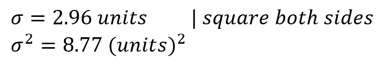 This means that each number of the set is on average 8.77 squared units away from the sample mean. If we try to graph it, it will look like this:
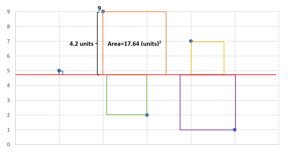
The figure above is a graphical representation of how to calculate population variance, which we will talk through.
- Each blue marker represents a data point.
- Step 1 is to find the mean value, which for this dataset is 4.8, depicted by the red line.
- Then, for each data point, subtract the data value from the mean to find its distance from the mean (9 – 4.8 = 4.2).
- Then, you have to square this value (4.2×4.2 (units) = 17.64 (units)^2).
- For each of the points, the size of the square represents the amount of variance which is the same whether a point is above or below the mean.
- Next, we have to sum the areas of the squares and finally divide them by the number of squares to calculate the overall we will get the variance – an average squared distance of each dataset constituent from the average line.
The variance tells us how variable the data is, as a squared value. This is less widely used than standard deviation (which is the linear equivalent of variance) as the standard deviation is in the same units as the mean.
Sample vs population variance and standard deviation
According to the American Lung Association, an estimated prevalence of lung cancer for 2020 in the USA was around 541,000. Should there be research investigating efficacy of a therapy in lung cancer patients in the USA, it would not be possible for all 541,000 patients to be enrolled in the research. Instead, only a representative number of the total number of patients would be enrolled. This representative subset of the lung cancer population is called a ‘sample’.
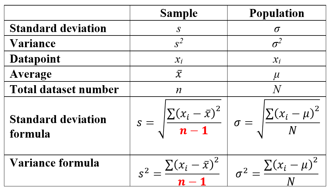
The formulae above for both standard deviation and variance were written as for a population, and not for a sample, although a substantial amount of research is actually conducted on samples representing population and not on a population itself. For this reason, (bio)statisticians use adjusted formulae to calculate standard deviation and variance of a sample. The key differences between these two formulae are listed in the table below:
Let’s look at this through an example…
If we take two studies which recruit people of different ages (in years):
| Group | Dataset |
| A | 65, 44, 52, 18, 46, 73, 25, 34, 46, 49, 53, 61 |
| B | 47, 51, 44, 39, 47, 50, 43, 49, 51, 40, 39, 52 |
- Which group of patients has a narrower spread of ages?
- Which group do you think would have greater chances to have internal validity but not external validity?
- If this study is of a disease that primarily affects the middle-aged population, which study would have a greater chance of achieving both internal and external validity?
Looking at the table below, Group A has a more diverse, variable dataset than Group B. Therefore, the results that come out of Group A have a greater chance that they will apply to all of the members of the dataset (internal validity).
We are looking for a study of middle-aged participants. The age range in Group B (39-52) is lower than in Group A (18-73). The results of Group B have greater chances of applying to the majority of patients suffering from this disease than the results of Group A (external validity), as well as to the patients from the study sample (internal validity).
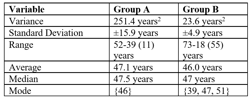
Furthermore, from the table, we can see that the measures of central tendency appear to be very similar between Group A and Group B. Yet, the variance and standard deviation are by far and large greater in Group A compared to Group B, indicating that the dataset has quite a large variability in its constituents. Hence, we can say that Group B has a more homogenous dataset than Group A.
Summary
- Variability is the extent to which data point diverge from the mean. It can be caused by either measurement errors, biological, or temporal causes.
- Measures of variability are statistical tools that help us assess data variability by informing us about the quality of a dataset mean.
- Range informs us about two end values of dataset; the minimum and the maximum value. On the other hand, standard deviation and variance describe how diverse our dataset is.
- Standard deviation is a linear measure of dataset spread around mean and thus it enables us to use and compare it with average, whilst variance is a non-linear measure of dataset.
- Regardless of that, as a rule of thumb, it is true for both standard deviation and variance that the greater they are, the greater variability of a dataset is.
- In research, these measures help us assess if a dataset meets internal and external validity; that is, it helps us understand if the results truthfully represent sample (internal validity) and population (external validity).
You can continue your learning in my next blog, which discusses the coefficient of variation and z-score.