A Brief Introduction to Statistical Averages
Posted on 14th April 2022 by Avishek Mukherjee

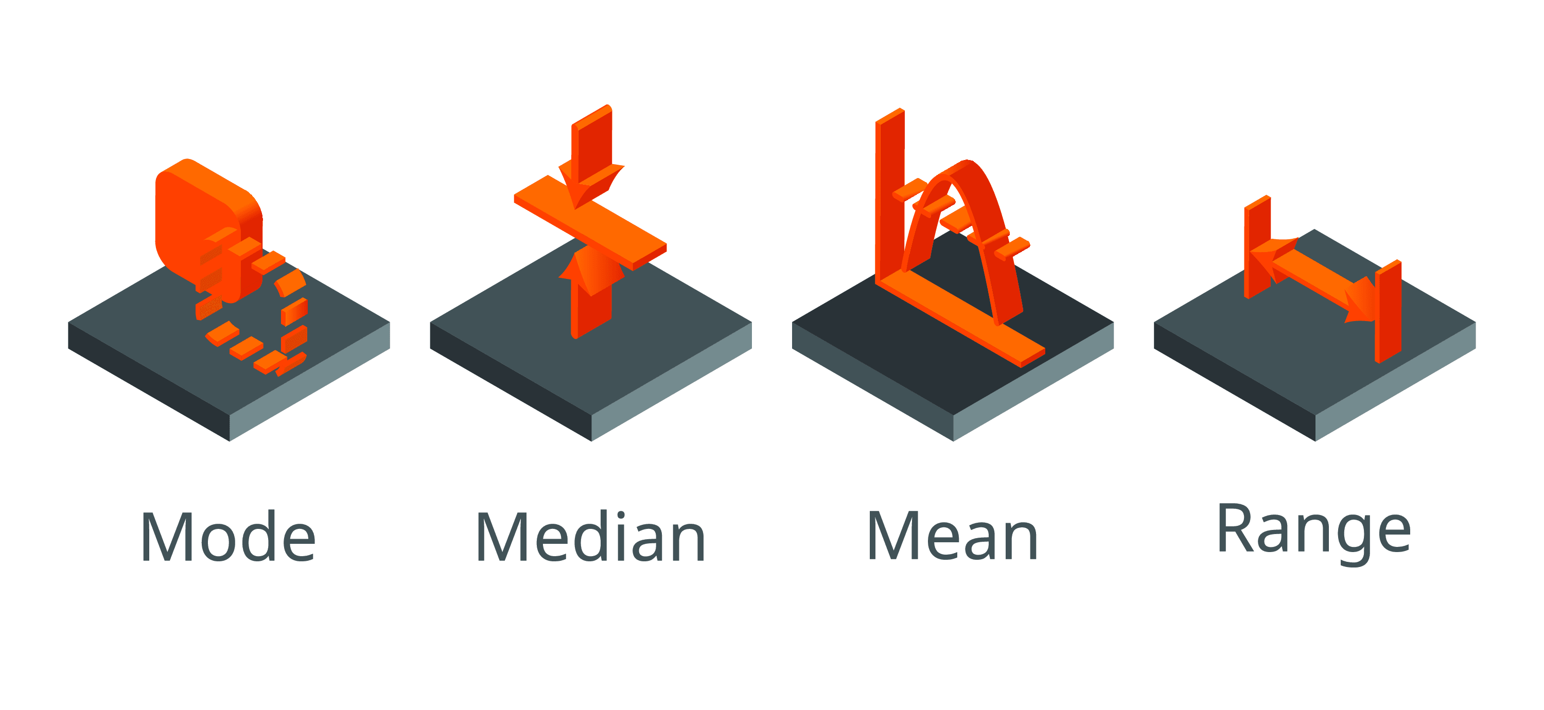
Statistical averages are a set of very useful tools used for data analysis. The word “average” implies a value in the distribution, around which other values are distributed. This tutorial aims to make is easier for those who find it difficult to understand the basic concepts of central tendency, as well as act as a go to resource for students who want to refresh their understanding on this topic.
The Mean
The arithmetic mean is widely used in statistical calculations. To obtain the mean of a set of data, the individual observations are added together, and then divided by the number of observations. Adding the individual observations is known as “Summation”. It is denoted by the symbol “S” or “Σ”. The individual observations are denoted by the symbol “η”, and the mean by the symbol “x̄” (popularly known as X bar).
An example of mean is calculated is as follows :
Suppose the fasting blood sugars (FBS) of 5 patients are 110, 98, 106,120, 114.
The summation comes out to 548.
The total number of observations are 5.
The mean is calculated by dividing 548 by 5, which results in 109.6.
Advantages of Mean
- It is very easy to calculate
- It is very easy to understand
Disadvantages of Mean
It may sometimes be influenced by abnormal values in the set of data.
For example, if the FBS of the last patient in the above distribution was 190, the mean would consequently come out to be 124.8, which is not a true reflection of the actual data.
Nevertheless, the arithmetic mean is by far the most useful of statistical averages.
The Median
The median is a different kind of average. It does not depend on the sum of the observations, or the number of observations. To ascertain the median, the data is first arranged in ascending or descending orders of magnitude. Then the middle observation is located. The value of the middle observation is the median.
To take an example, the diastolic blood pressures of 7 individuals are :
83, 75, 81, 79, 71, 95, 75.
When we arrange the data in ascending order,
71, 75, 75, 79, 81, 83, 95.
The central value and consequently the median here is 79.
If there are an even number of observations, then the median is worked out by taking the average of the two middle values.
For example, if the diastolic blood pressure of 8 individuals is taken :
83, 75, 81, 79, 71, 95, 75, 77.
Arranging the data in ascending order :
71, 75, 75, 77, 79, 81, 83, 95
Thus the median comes out to be (77+79)/2 = 78
Advantage of Median over Mean
Any abnormal value in the distribution does not affect the median, whereas the mean is seriously affected. Thus, the median is nearer to the truth, and therefore more representative than the mean.
The Mode
The mode is the most commonly occurring value in a distribution of data.
For example, the HbA1c (average blood glucose (sugar) levels for the last two to three months) of 10 different patients are as follows :
5.8, 5.7, 6.3, 6.0, 5.9, 5.7, 6.6, 6.2, 5.7, 5.9
The mode or the most frequently occurring data is 5.7.
Advantages of Mode
- It is easy to understand
- It is not affected by the extreme values in a data set
Disadvantages of Mode
- The exact location of the value of mode is often uncertain
- It is often not clearly defined
Thus, mode is not regularly used in medical or biological statistics.
References
- Park’s Textbook of Preventive and Social Medicine – K. Park (MBBS, MS)/ Twenty-sixth Edition. [M/s Banarsidas Bhanot Publishers]
You may also be interested in these other blogs relating to the topic:
Measures of central tendency in clinical research papers: what we should know whilst analysing them
A beginner’s guide to standard deviation and standard error


